Spatial Filtering and Convolution
The neighbourhood operation that underpins blurring, sharpening, edge detection, and the first layer of every convolutional network.
Convolution slides a small matrix over the image, multiplies it elementwise with the pixels underneath, and writes the sum to the output. Change the numbers in the matrix and the same loop blurs, sharpens, or finds edges.
2D Discrete Convolution
J(x, y) = Σᵢ Σⱼ k(i, j) · I(x − i, y − j)(3.1)Note the subtraction. True convolution flips the kernel; correlation does not. For symmetric kernels the two are identical, which is why the distinction is often ignored until it matters.
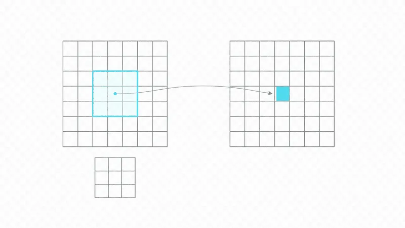
Image prompt
Minimal technical diagram on a transparent background. Left: an 8 by 8 grid of squares in thin grey stroke with a 3 by 3 sub-window outlined in cyan and lightly filled. Right: a second 8 by 8 grid, mostly empty, with a single square filled cyan at the position corresponding to the window centre. A thin arrow curves from the window to that square. Below the left grid, a small 3 by 3 matrix of empty cells representing the kernel. No text, no numbers, flat vector, 1.5px strokes, generous negative space, 16:9.
Boundary handling
At the border the window hangs off the edge of the image. Every strategy for filling those positions is a guess, and each guess produces a characteristic artefact.
| Strategy | Behaviour | Artefact |
|---|---|---|
| Zero pad | Treat outside as black | Dark vignette on blurred edges. |
| Clamp | Repeat the edge pixel | Smearing of edge colour outward. |
| Mirror | Reflect across the border | Usually invisible, the safe default. |
| Wrap | Sample from the opposite side | Correct only for tiling textures. |
| Crop | Shrink the output | No artefact, but the size changes. |
Smoothing and Noise Reduction
Box and Gaussian
A box blur averages the window uniformly. It is fast and it rings, because a rectangle in the spatial domain is a sinc in the frequency domain. A Gaussian weights by distance from the centre and does not ring, which is why it is the default smoothing kernel everywhere.
The three by three Gaussian approximation. The centre tap is highlighted.
Median
The median filter sorts the window and takes the middle value. It is not a convolution, because sorting is not linear, and that nonlinearity is exactly what makes it remove salt and pepper noise while leaving edges intact. An outlier pixel cannot drag the median the way it drags a mean.
Bilateral
The bilateral filter weights neighbours by two distances at once: how far away they are, and how different their values are. Pixels across an edge get a low weight and therefore do not bleed. The cost is high and the result is the smooth-but-sharp look now associated with mobile photography.
w(i, j) = exp( −d²/2σ_s² ) · exp( −Δ²/2σ_r² )(3.2)σ_s is the spatial radius, σ_r the range tolerance. Raising σ_r far enough turns the bilateral filter back into a Gaussian.
Edge Detection and Sharpening
An edge is a place where intensity changes quickly. First derivatives locate it by magnitude, second derivatives locate it by zero crossing. Both amplify noise, so both are preceded by smoothing.
Sobel horizontal gradient. The vertical operator is its transpose.
The four-neighbour Laplacian, a second derivative in a single kernel.
The Canny pipeline
Canny is not an operator, it is a sequence. Each stage removes a specific failure of the naive gradient approach.
- 01
Gaussian smoothing
Suppresses noise that would otherwise register as gradient. The chosen sigma sets the scale of the edges that survive.
- 02
Gradient magnitude and direction
Sobel in both axes gives a vector per pixel. Magnitude says how strong, direction says which way the edge runs.
- 03
Non-maximum suppression
Thin the ridge to one pixel by discarding any sample that is not a local maximum along the gradient direction.
- 04
Hysteresis thresholding
Two thresholds. Strong pixels are kept, weak pixels are kept only if connected to a strong one. This is what produces continuous contours instead of dashes.
Unsharp masking
Sharpening is subtraction. Blur a copy, subtract it from the original to isolate the detail, then add that detail back with a gain. The name comes from darkroom practice, where the blurred copy really was an unsharp negative.
J = I + amount · (I − blur(I, σ))(3.3)σ sets which frequencies are treated as detail. amount sets how much of it returns. A threshold on the difference prevents noise from being sharpened alongside the subject.
Module 04 stops changing values and starts moving them, which introduces a problem convolution never had: the destination coordinate is rarely an integer.