Foundations of Digital Images
What a pixel is, where it came from, and how a grid of them sits in memory. Everything later in the handbook is an operation on this structure.
An image is a measurement. Before it is an array it is a count of photons that struck a small square of silicon during a short interval, converted to a voltage, and then rounded to an integer. Two decisions govern that conversion, and both of them throw information away permanently.
Analog to Digital
The scene in front of a lens is continuous in space and in intensity. A sensor is discrete in both. Sampling handles the spatial axis, quantisation handles the intensity axis, and the artefacts they produce look nothing alike.
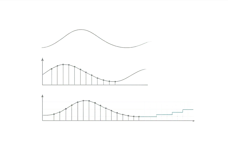
Image prompt
Minimal technical diagram on a transparent background, three stacked panels sharing one horizontal axis. Top panel: a smooth continuous sine-like curve in thin grey stroke. Middle panel: the same curve overlaid with evenly spaced vertical sample lines terminating in small dots on the curve. Bottom panel: a stepped staircase approximation of the curve in cyan, showing values snapped to discrete horizontal levels drawn as faint dotted guides. No text, no axis labels, flat vector, 1.5px strokes, generous spacing between panels, 16:8 aspect ratio.
Sampling
Sampling replaces a continuous field with values at regular positions. The sampling rate has to exceed twice the highest spatial frequency present, or detail above that limit folds back into the image as false low-frequency structure. That folding is aliasing, and it is the reason a striped shirt turns into a moiré pattern on video.
f_s > 2 · f_max(1.1)The Nyquist condition. Optical low-pass filtering before the sensor, or a blur before downsampling, is how the condition is enforced in practice.
Quantisation
Quantisation maps a continuous intensity onto a finite set of levels. With 8 bits there are 256 of them per channel. That is enough for most photographic content and not enough for a smooth gradient, where the boundaries between levels become visible as banding.
Dithering trades banding for noise by adding a small random or patterned offset before rounding. The error is still there, but it is spread across frequencies the eye tolerates better.
Anatomy of an Image
Three numbers describe the shape of any raster image: how many samples across, how many samples down, and how many values per sample. A fourth, the bit depth, describes the precision of each value.
| Property | Typical values | What it controls |
|---|---|---|
| Spatial resolution | 1920 × 1080, 4096 × 4096 | How much detail can be represented at all. |
| Channels | 1, 3, 4 | Grey, colour, or colour with transparency. |
| Bit depth | 8, 10, 16, 32 | Tonal precision and headroom for intermediate maths. |
| Alpha mode | Straight or premultiplied | Whether colour has been scaled by opacity already. |
Colour Spaces and Conversions
A colour space is a coordinate system for colour. Choosing the right one turns hard problems into easy ones. Selecting a skin tone is awkward in RGB and straightforward in a space where hue is one of the axes.
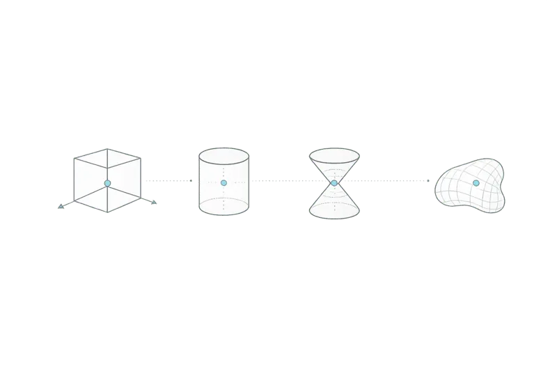
Image prompt
Four minimal wireframe solids arranged in a row on a transparent background: a cube labelled by its axes only through colour, a cylinder, a double cone, and an irregular blob shape. Each drawn in thin 1.5px grey lines with a single small cyan dot placed at the same relative interior position in every solid, connected between solids by a faint dotted line. Isometric perspective, flat vector, no text, no fill, generous negative space, 16:9.
RGB, HSL and HSV
RGB is additive and device oriented. HSL and HSV are cylindrical rearrangements of the same cube, built so that hue, saturation and lightness become separable. Neither is perceptually uniform, and both are cheap to compute, which is why they remain the default for interactive colour selection.
YCbCr and YUV
Splitting luma from chroma exploits a fact about human vision: spatial acuity for brightness is far higher than for colour. Encoders subsample the chroma planes, commonly to half resolution in both directions, and most viewers never notice.
| Scheme | Chroma resolution | Bytes per 4 pixels | Used by |
|---|---|---|---|
| 4:4:4 | Full | 12 | Mastering, screen capture, graphics. |
| 4:2:2 | Half horizontally | 8 | Broadcast, professional video. |
| 4:2:0 | Half in both axes | 6 | JPEG, H.264, most delivery formats. |
CIE LAB and LCH
LAB was designed so that equal numerical distances correspond roughly to equal perceived differences. That property makes it the right space for measuring colour error, for palette generation, and for any operation where two results need to be compared rather than merely computed. LCH is LAB in polar coordinates, which restores an intuitive hue axis.
Matrix-based conversions
Conversions between linear spaces are a single three by three matrix multiply. Conversions involving a nonlinear space add a transfer function on each side. Getting the order wrong is a quiet bug: colours end up close enough to look plausible and far enough to fail a comparison.
- 01
Decode the transfer function
Remove the sRGB curve to reach linear light. Skipping this step is the most common cause of over-saturated blends.
- 02
Apply the matrix
One three by three multiply moves the linear triple into the target primaries, for example sRGB to XYZ.
- 03
Encode the target transfer function
Apply the destination curve, then quantise. Rounding once at the end preserves more precision than rounding at each stage.
Memory and Data Structures
How pixels are arranged in memory determines how fast every later operation runs. Interleaved layouts keep a pixel contiguous. Planar layouts keep a channel contiguous. The first suits per-pixel work, the second suits per-channel work and vectorised code.
offset = y · stride + x · bytesPerPixel(1.2)Stride is not always width times bytes per pixel. Decoders pad rows to alignment boundaries, and reading past the visible width returns padding, not image data.
// Interleaved RGBA, the layout returned by CanvasRenderingContext2D.
const data = new Uint8ClampedArray(width * height * 4);

// Planar Float32, convenient for GPU upload and per-channel maths.
const r = new Float32Array(width * height);
const g = new Float32Array(width * height);
const b = new Float32Array(width * height);Module 02 takes this structure and starts changing values, one pixel at a time, without reference to any neighbour.