Frequency Domain Processing
Describing an image by the spatial frequencies it contains, and the class of problems that becomes trivial once you do.
Any image can be written as a sum of sinusoids of different frequencies, orientations and phases. The Fourier transform computes that decomposition. Nothing is lost and nothing is added, but problems that are awkward in the spatial domain sometimes become a single multiplication.
Fast Fourier Transform
The discrete Fourier transform is defined as a double sum over the whole image, which costs O(N²) per axis. The fast Fourier transform computes the same result in O(N log N) by exploiting the redundancy in that sum. For a megapixel image the difference is between minutes and milliseconds.
F(u, v) = Σₓ Σᵧ I(x, y) · e^(−2πi(ux/W + vy/H))(5.1)The output is complex and the same size as the input. Low frequencies land near the origin, which is why spectra are usually shifted so the origin sits at the centre.
Amplitude and phase
Every coefficient carries two numbers. Amplitude says how much of that frequency is present. Phase says where it sits. Amplitude spectra are the ones people publish, and phase is the one that actually carries the structure. Reconstructing an image from one image’s amplitude and another’s phase yields the second image, faintly.
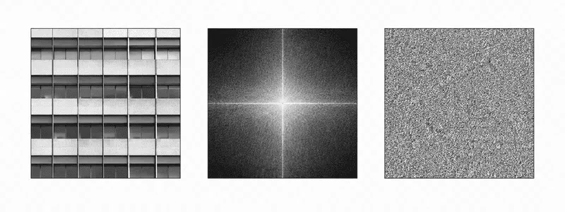
Image prompt
Three square panels in a row on a transparent background. Panel one: a simple grey photographic scene of a building facade with strong horizontal and vertical lines. Panel two: its Fourier amplitude spectrum, a dark square with a bright central point and bright orthogonal streaks radiating horizontally and vertically, rendered in greyscale with a faint cyan tint at the centre. Panel three: an unrecognisable field of grey noise with the same overall texture statistics. Thin 1px borders around each panel, no text, generous spacing, 16:6.
Frequency Filtering
A frequency filter is a mask multiplied against the spectrum. Zero out the outer region and high frequencies disappear, which is a blur. Zero out the centre and only edges remain.
- 01
Pad to a friendly size
Radix-2 implementations want power-of-two dimensions. Pad with mirrored content rather than zeros to avoid a hard discontinuity at the seam.
- 02
Transform and shift
Run the forward FFT, then swap quadrants so the zero frequency sits at the centre. Every mask below assumes that layout.
- 03
Multiply by the mask
Use a smooth mask. A hard circular cutoff produces concentric ringing in the result, the same overshoot seen with sharp resampling kernels.
- 04
Inverse transform and crop
Take the real part, discard the padding, and clamp. Small imaginary residue is numerical noise, not signal.
| Filter | Mask shape | Effect |
|---|---|---|
| Low-pass | Passes the centre | Smoothing, noise reduction. |
| High-pass | Blocks the centre | Edge isolation, detail extraction. |
| Band-pass | Passes an annulus | Texture analysis at one scale. |
| Notch | Blocks isolated points | Removal of a single periodic pattern. |
Band-pass and notch filters
Periodic noise is the case where the frequency domain earns its keep. Scanner banding, halftone screens from printed originals, and interference patterns all appear in the spectrum as small bright spots away from the centre. Suppress those spots and the pattern vanishes from the image while the rest of the content stays untouched.
Doing the same job spatially would require a filter tuned to the exact period and orientation of the pattern. In the frequency domain it is a handful of small discs.
Module 06 returns to the spatial domain with a different question: not what values the pixels hold, but what shapes they form.