Geometry and Interpolation
Moving pixels to new positions, and deciding what value belongs at a coordinate that falls between samples.
Every geometric operation splits into two independent questions. Where does each output pixel come from, and what value should it take given that the source position is almost never an integer. The first question is linear algebra. The second is resampling, and it is where quality is won or lost.
Affine and Perspective Mapping
An affine transform preserves parallel lines. Translation, scaling, rotation and shear are all affine, and all four compose into a single three by three matrix applied to homogeneous coordinates.
[x']   [a  b  tx] [x]
[y'] = [c  d  ty] [y]
[1 ] [0 0 1] [1](4.1)Composition is matrix multiplication, and it is not commutative. Rotating then translating places the subject somewhere quite different from translating then rotating.
Homography
A perspective transform relaxes the parallel-line guarantee. The bottom row of the matrix stops being fixed, the result is divided by the third component, and a rectangle can map to any convex quadrilateral. Eight degrees of freedom, four point correspondences, one linear solve.
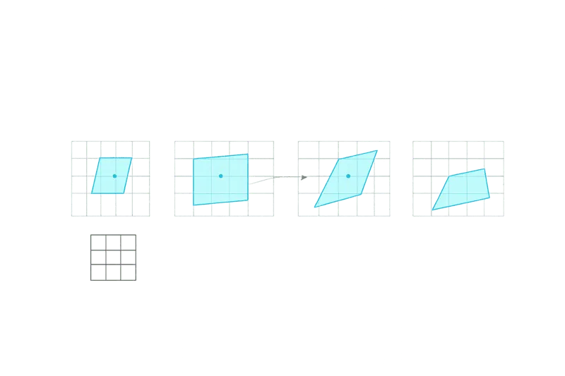
Image prompt
Five minimal panels in a row on a transparent background. Each panel shows a faint dashed grey unit square and, overlaid, a solid cyan quadrilateral that is its transform: panel one translated, panel two scaled, panel three rotated, panel four sheared, panel five a trapezoid with converging sides for perspective. Thin 1.5px strokes, no fill, no text, flat vector, equal spacing, 16:6 aspect ratio.
Interpolation Algorithms
The inverse transform lands at a fractional coordinate. Interpolation decides what value that position holds, and the choice of method is a direct trade of sharpness against cost against artefacts.
| Method | Taps | Character | Use for |
|---|---|---|---|
| Nearest neighbour | 1 | Blocky, preserves exact values | Masks, labels, pixel art. |
| Bilinear | 4 | Soft, no ringing | Real-time work, GPU default. |
| Bicubic | 16 | Sharper, slight ringing | General photographic resizing. |
| Lanczos 3 | 36 | Sharpest, visible ringing | Downscaling where detail matters. |
Nearest neighbour and bilinear
Nearest neighbour rounds the coordinate and copies. It never invents a value, which matters when the pixel values are category identifiers rather than intensities. Interpolating a segmentation mask produces labels that do not exist.
v = (1−u)(1−t)·p₀₀ + u(1−t)·p₁₀ + (1−u)t·p₀₁ + u·t·p₁₁(4.2)Bilinear interpolation as two linear interpolations. u and t are the fractional parts of the source coordinate.
Bicubic and Lanczos
Both fit a smooth function through a wider neighbourhood. Both have negative lobes, which is what makes them sharper than bilinear and also what makes them overshoot at hard edges. The overshoot is the ringing you see as a faint light line beside a dark boundary.
A one dimensional resampling kernel written as a column. Negative outer taps are what produce both the extra sharpness and the ringing.
Image prompt
Two versions of the same downscaled photograph for a before and after slider. Subject: a brick facade with a fine metal railing and lettering on a sign, framed straight on, high detail. Version A: downscaled with a soft kernel, mortar lines mushy, railing partly dissolved. Version B: identical framing downscaled with a sharp kernel, mortar lines crisp, railing distinct, faint bright fringing beside the darkest edges. Photographic, neutral daylight, no people, identical composition, 16:9.
Practical Applications
Three everyday tasks fall out of the same machinery.
Cropping is a translation followed by a size change, and it needs no resampling at all if the crop rectangle lands on integers. Horizon alignment is a rotation about the image centre, followed by a crop that removes the corners the rotation exposed. Lens distortion correction is the odd one out: the mapping is not a matrix but a radial polynomial, so it is applied per pixel rather than composed.
r_corrected = r · (1 + k₁r² + k₂r⁴ + k₃r⁶)(4.3)The standard radial model. Positive k₁ corrects barrel distortion, negative corrects pincushion. Coefficients come from a calibration pass, not from inspection.
Module 05 changes basis entirely. Instead of describing an image by position, it describes it by frequency.