Introduction
A field guide to digital image processing, written for people who ship image code rather than for people who only read about it.
Image processing sits in an awkward place. The mathematics is old and settled, the libraries are excellent, and yet almost every project runs into the same handful of problems: a resize that softens detail, a filter that crawls on large inputs, a colour shift nobody can explain. This handbook is written for those moments.
The nine modules move from the physics of capture to the neural models that now sit at the end of many pipelines. Along the way they keep returning to one question. What is actually happening to the numbers?
What this covers
Each module is a self-contained treatment of one layer of the stack. The ordering is deliberate, because later modules assume the vocabulary of earlier ones, but nothing stops you from opening Module 05 on a Tuesday afternoon because a periodic pattern turned up in a scan.
The data itself
Sampling, quantisation, channel layout, colour spaces, memory strides, and everything you can do to a single pixel without looking at its neighbours.
Operators
Convolution, geometric mapping, the frequency domain, and morphology. This is the classical core of the field.
Storage
How the array becomes a file, what the encoder throws away, and why two visually identical images can differ by an order of magnitude in size.
Execution
Where the work runs. Typed arrays, shaders, workers, WebAssembly, and the learned models that replace hand-written kernels.
How to read it
Every section follows the same rhythm: the idea in plain language, the operation written out, a figure, and then the failure modes. The failure modes matter most. Textbooks tend to show the clean case, and production images are rarely clean.
- 01
Read the operation before the code
Most bugs in image pipelines are conceptual. A wrong colour space or an off-by-one in the kernel centre will not look like a bug, it will look like a slightly disappointing result.
- 02
Reproduce on a small array
A five by five test image with hand-written values will expose boundary and rounding errors that a photograph hides completely.
- 03
Measure before optimising
Module 08 covers the tools. Reach for them after the correct result exists, not before.
The working environment
Code samples assume a browser environment with Canvas, ImageData, and typed
arrays available, and they avoid framework dependencies. Where a native tool is
the right answer, it is named. Nothing in the handbook depends on a specific
library version.
A note on figures
Figures in this handbook carry their generation brief with them. Open the prompt panel under any figure to see exactly what the illustration is meant to show. Placeholders stay in place until the artwork is produced, so the page structure never depends on assets that do not exist yet.
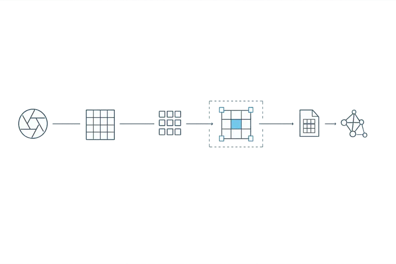
Image prompt
Minimal horizontal flow diagram on a transparent background. Six evenly spaced nodes connected by a single thin line: a lens aperture, a sensor grid, a pixel array, a convolution window, a compressed file block, a neural network graph. Each node drawn as a simple geometric glyph in thin 1.5px strokes, monochrome grey, with the fourth node accented in cyan. Generous negative space, no text, no shadows, no gradients. Flat vector, technical drawing aesthetic, 16:7 aspect ratio.
The next page fixes the notation used throughout. It is short, and skipping it will cost you time later.