Point Operations and Histograms
Operations where the output pixel depends only on the input pixel at the same position. Cheap, parallel, and responsible for most of what people call editing.
A point operation is a function applied independently to every sample. It has no notion of neighbourhood, shape, or edge. That restriction makes it trivially parallel and, for 8-bit data, precomputable into a table of 256 entries.
Pixel-wise Transformations
Brightness adds a constant. Contrast scales around a pivot. Inversion subtracts from the maximum. Written as one expression they are the same operation with different coefficients.
J(x, y) = clamp(a · I(x, y) + b)(2.1)a controls contrast, b controls brightness. Clamping is what makes the operation lossy: values pushed past the range do not come back.
Gamma correction and LUTs
Gamma correction raises the normalised value to a power. Because the operation depends on nothing but the input value, it collapses into a lookup table built once and applied with a single array read per sample.
// Build once, apply per pixel.
const lut = new Uint8Array(256);
for (let v = 0; v < 256; v++) {
  lut[v] = Math.round(255 * Math.pow(v / 255, 1 / gamma));
}

for (let i = 0; i < data.length; i += 4) {
  data[i] = lut[data[i]];
  data[i + 1] = lut[data[i + 1]];
  data[i + 2] = lut[data[i + 2]];
}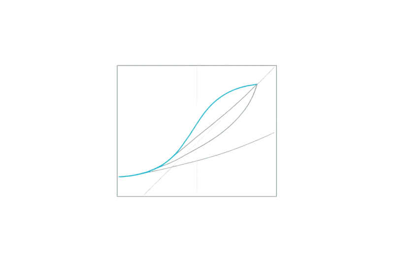
Image prompt
Minimal line chart on a transparent background inside a square plotting area with thin grey border and a faint diagonal identity line. Four smooth curves drawn in 1.5px strokes: an S-shaped contrast curve in cyan, a concave gamma curve in grey, a convex inverse-gamma curve in grey, and a descending straight inversion line in light grey. No text, no tick labels, no grid beyond four faint interior guides, flat vector, generous margin around the plot, 16:9.
Histogram Analysis
A histogram counts how many pixels fall into each intensity bin. It discards all spatial information and keeps all tonal information, which makes it the right tool for exposure decisions and the wrong tool for anything about shape.
| Shape | Reading | Usual response |
|---|---|---|
| Bunched at the left | Underexposed or very dark subject | Lift midtones, check for crushed shadows. |
| Bunched at the right | Overexposed, possible clipping | Nothing recovers clipped highlights. |
| Narrow central peak | Low contrast, flat scene | Stretch, or equalise if detail is hidden. |
| Two separated peaks | Foreground and background differ strongly | A global threshold will work well. |
Global equalisation
Equalisation redistributes intensities so the cumulative distribution becomes approximately linear. Detail hidden inside a narrow band of values becomes visible. Noise hidden in the same band becomes visible too.
J(x, y) = round( (L − 1) · cdf( I(x, y) ) )(2.2)cdf is the normalised cumulative histogram. The transform is itself a lookup table, so the cost is one pass to build and one pass to apply.
CLAHE
Contrast Limited Adaptive Histogram Equalisation runs the same idea on tiles rather than on the whole frame, clips each tile histogram at a ceiling to stop noise amplification, and interpolates between neighbouring tiles to avoid visible seams. It is the version that survives contact with real photographs.
Image prompt
Two versions of the same photograph for a before and after slider. Subject: a stone archway opening onto a bright courtyard, shot from inside so the interior is deep shadow and the exterior is near clipping. Version A: flat, unprocessed, shadow detail invisible, exterior blown out. Version B: identical framing and colour, with local contrast recovered so the stone texture in shadow and the courtyard detail are both legible. Photographic, neutral colour, no people, no text, identical composition between the two, 16:9.
Thresholding and Binarisation
Thresholding reduces an image to two classes. The difficulty is never the comparison, it is choosing the value to compare against.
| Method | How the threshold is chosen | Fails when |
|---|---|---|
| Fixed | Set by hand or by convention | Lighting changes between inputs. |
| Otsu | Maximises between-class variance over the histogram | The histogram is not bimodal. |
| Adaptive mean | Local window mean minus a constant | The window is smaller than the features. |
| Adaptive Gaussian | Weighted local mean | Noise dominates the window. |
Adaptive methods cost a neighbourhood pass, which strictly speaking makes them spatial filters. They are grouped here because the decision is still per pixel.
Module 03 lifts the independence restriction. Once a pixel is allowed to consult its neighbours, the entire classical toolkit opens up.